Raster Conversion
Three bands are read from an image. Then we do some raster conversion on it. This new bands are then written to a new multi band TIFF.
At first import rasterpy. ..
import rasterpy as rpy
import numpy as np
After that we define a path where our test tif file is located. ..
path = ".\\rasterpy\\tests\data"
Then we open the grid and read it to an multidimensional array: ..
grid = rpy.Raster('RGB.BRF.tif', path)
The quantification factor is a factor which scales reflectance value between 0 and 1. For sentinel 2 the factor is 10000 ..
grid.to_array(flatten=False, quantification_factor=10000)
By default the loaded grid is flatten. The reason is as following: With a flatten 2 dimensional array the calculations based on the array are much easier. But in our case this is not necessary: ..
>>> print(grid.array)
[[[0.1049 0.0979 0.1047 ... 0.0469 0.0551 0.0553]
  [0.1008 0.0974 0.0984 ... 0.0449 0.0497 0.0574]
  [0.1039 0.0957 0.1002 ... 0.0477 0.0546 0.0653]
  ...
  [0.1226 0.1151 0.1363 ... 0.0641 0.0599 0.0643]
  [0.1136 0.1299 0.144  ... 0.0654 0.0625 0.0651]
  [0.1069 0.1034 0.1356 ... 0.0616 0.0546 0.0629]]
 [[0.1025 0.0968 0.1027 ... 0.0435 0.0567 0.0585]
  [0.1008 0.0943 0.0996 ... 0.0466 0.0531 0.0625]
  [0.0969 0.0929 0.0987 ... 0.0523 0.0604 0.0692]
  ...
  [0.1223 0.112  0.1367 ... 0.0683 0.0587 0.0621]
  [0.112  0.1282 0.1409 ... 0.0658 0.0591 0.0635]
  [0.106  0.1018 0.1394 ... 0.0616 0.0551 0.0588]]
 [[0.1146 0.1088 0.114  ... 0.0484 0.0644 0.0703]
  [0.1112 0.1076 0.1148 ... 0.048  0.0599 0.0773]
  [0.1125 0.1064 0.1119 ... 0.0564 0.0747 0.0886]
  ...
  [0.1381 0.1259 0.1473 ... 0.0873 0.0746 0.0746]
  [0.1268 0.1404 0.1624 ... 0.0782 0.0702 0.0758]
  [0.1207 0.1194 0.1543 ... 0.0752 0.0617 0.0678]]]
Now we convert the whole file from a Bidirectional Reflectance Factor (BRF) into a Bidirectional Reflectance Distribution Function (BRDF): ..
grid.convert(system='BRF', to='BRDF', output_unit='dB')
After that we can write the converted data as a multi band tiff: ..
grid.write(data=grid.array, filename='RGB.BRDF.tif', path=path)
We can also convert the arrays from a BRF or BRDF into Backscatter coefficients (BSC). For this we need the inclination (iza) and viewing (vza) angles. These information is in the first two bands of the dataset. Thus, we specify it with parameter band=(1, 2): ..
angle = rpy.Raster('RGB.BRF.Angle.tif')
angle.to_array(band=(1, 2), flatten=False)
Note, that the arrays were converted from a BRF into a BRDF (dB) in the previous step: ..
grid.convert(system='BRDF', to='BSC', system_unit='dB', output_unit='dB', iza=angle.array[0], vza=angle.array[1])
After the conversion we can wrtie the array to a raster file: ..
grid.write(data=grid.array, filename='RGB.BSC.tif', path=path)
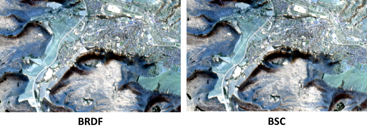
The result is